R 3D plot
R has several functions can plot 3D images, such as persp() function, package scatterplot3d and rgl.
persp(x = seq(0, 1, length.out = nrow(z)),
y = seq(0, 1, length.out = ncol(z)),
z, xlim = range(x), ylim = range(y),
zlim = range(z, na.rm = TRUE),
xlab = NULL, ylab = NULL, zlab = NULL,
main = NULL, sub = NULL,
theta = 0, phi = 15, r = sqrt(3), d = 1,
scale = TRUE, expand = 1,
col = "white", border = NULL, ltheta = -135, lphi = 0,
shade = NA, box = TRUE, axes = TRUE, nticks = 5,
ticktype = "simple", ...)
theta, phi: angles defining the viewing direction. theta gives the azimuthal direction and phi the colatitude.
r: the distance of the eyepoint from the centre of the plotting box.
d: a value which can be used to vary the strength of the perspective transformation. Values of d greater than 1 will lessen the perspective effect and values less and 1 will exaggerate it.
scale: before viewing the x, y and z coordinates of the points defining the surface are transformed to the interval [0,1]. If scale is TRUE the x, y and z coordinates are transformed separately. If scale is FALSE the coordinates are scaled so that aspect ratios are retained. This is useful for rendering things like DEM information.
expand: a expansion factor applied to the z coordinates. Often used with 0 < expand < 1 to shrink the plotting box in the z direction.
border: the color of the line drawn around the surface facets. The default, NULL, corresponds to par("fg"). A value of NA will disable the drawing of borders: this is sometimes useful when the surface is shaded.
ltheta, lphi: if finite values are specified for ltheta and lphi, the surface is shaded as though it was being illuminated from the direction specified by azimuth ltheta and colatitude lphi.
shade: the shade at a surface facet is computed as ((1+d)/2)^shade, where d is the dot product of a unit vector normal to the facet and a unit vector in the direction of a light source. Values of shade close to one yield shading similar to a point light source model and values close to zero produce no shading. Values in the range 0.5 to 0.75 provide an approximation to daylight illumination.
box: should the bounding box for the surface be displayed. The default is TRUE.
axes: should ticks and labels be added to the box. The default is TRUE. If box is FALSE then no ticks or labels are drawn.
ticktype: character: "simple" draws just an arrow parallel to the axis to indicate direction of increase; "detailed" draws normal ticks as per 2D plots.
nticks: the (approximate) number of tick marks to draw on the axes. Has no effect if ticktype is "simple".
Let's try to plot z = 4x + 3y - 12;
> x <- seq(-5,5,length = 100)
> y <- seq(2,24,length = 100)
> fun <- function(x,y){
+ return (4 * x + 3 * y -12)
+ }
> z <- outer(x,y,fun)
> persp(x,y,z,col="green",theta=45,phi=30,expand=0.8,ticktype="detailed")

cloud() and wireframe() of "lattice" package also support 3D plotting.
> library(lattice)
> x <- seq(-3,3,by=0.4)
> y <- seq(-3,3,by=0.4)
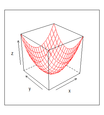
> fun <- function(x,y) {x * x + y * y}
> z <- outer(x,y,fun)
> wireframe(z,xlab="x",ylab="y",col="red")

> z <- outer(x,y,FUN = function(x,y){x * x * y})
> cloud(z ~ x * y, screen = list(z = 14, x = -75, y = 4))

Package "rgl" is widely used for interactive 3D plotting.
> install.packages("rgl", repo = "http://cran.r-project.org",dep = TRUE)
> library(rgl)
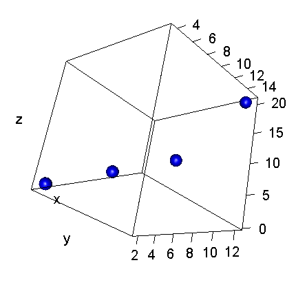
> a <- matrix(c(2,5,8,12,4,8,12,15,1,5,9,20),nrow=4,ncol=3,dimnames=list(c(1,2,3,4),c("x","y","z")))
> a
   x  y  z
1  2  4  1
2  5  8  5
3  8 12  9
4 12 15 20
> plot3d(a,type="s",col="blue")

You can rotate the picture in whatever angle like following:

The picture can be saved:
> rgl.snapshot(filename="d:/tp.png",fmt="png")
persp3d() is another function in the package to draw surfaces similar to the classic persp() function.
> x <- seq(-3,3,by=0.1)
> y <- seq(-3,3,by=0.1)
> z <- outer(x,y,FUN=function(x,y){x*x*x*x/2 - y * y * y/5})
> persp3d(z, col="yellow",xlab="x",ylab="y")

R package "scatterplot3d" can be used to draw 3D scatter plots, to install this package:
> install.packages("scatterplot3d",repos="http://cran.r-project.org",dep=TRUE)
> library(scatterplot3d)
Following is the data file:
Let first read in the data from the file:
> x <- read.csv("scatterplot.csv",header=T,sep="\t")
> x <- t(x)
> ex <- as.numeric(x[2,1:ncol(x)])
> qu <- as.numeric(x[3,1:ncol(x)])
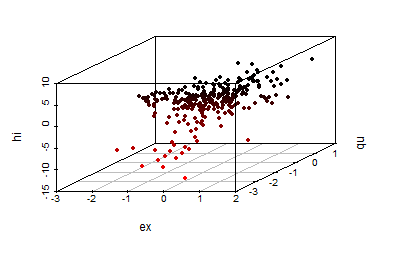
To draw a 3D scatter plot based on the "Expression", "Quality" and "Height" values:
> hi <- as.numeric(x[4,1:ncol(x)])
> scatterplot3d(ex,qu,hi,pch=20,highlight.3d=T)

We can add more parameters like:
> scatterplot3d(ex,qu,hi,pch=20,highlight.3d=T,type="h")


