R binomial distribution

Density, distribution function, quantile function and random generation for the binomial distribution with parameters size and prob.

rbinom(n, size, prob)
dbinom(x, size, prob, log = FALSE)
pbinom(q, size, prob, lower.tail = TRUE, log.p = FALSE)
qbinom(p, size, prob, lower.tail = TRUE, log.p = FALSE)

x, q: vector of quantiles.
p: vector of probabilities, 0 < p < 1.
n: number of observations. If length(n) > 1, the length is taken to be the number required.
size: number of trials (zero or more).
prob: probability of success on each trial.
log, log.p: logical; if TRUE, probabilities p are given as log(p).
lower.tail: logical; if TRUE (default), probabilities are P[X ≤ x], otherwise, P[X > x].

rbinom() generates random sequences of binomial or multinomial distribution. For example, let's flip coins. Each run has 40 flips (size), each flip has 10% chance of head (probability of success), and size * probability is the generated success number of the run, altogether 20 runs.

> rbinom(20,40,0.1)
 [1] 5 4 3 4 3 7 3 5 4 3 2 1 5 5 4 5 2 3 3 5

Let's expect each flip has 90% chance of head:

> rbinom(20,40,0.9)
 [1] 36 36 37 33 37 37 35 37 37 34 36 35 39 36 38 38 37 37 32 39

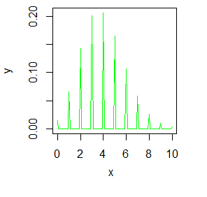
dbinom() for binormal distribution probability density analysis.

> x <- seq(0,10, by = 0.1)
> y <- dbinom(x,40,0.1)
There were 50 or more warnings (use warnings() to see the first 50)
> plot(x,y,type="l",col="green")

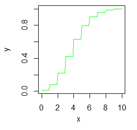
pbinom() for binomial distribution cumulative probability density analysis:

> y <- pbinom(x,40,0.1)
> plot(x,y,type="l",col="green")

qbinom() gets the value of quantile of binomial distribution.

> qbinom(0.05,40,0.1)
[1] 1
> qbinom(0.95,40,0.1)
[1] 7

binom.test() performs binomial test of null hypothesis about binomial distribution.